Test of a cheap power bank

Introduction
I got a small aluminium power bank (Figure 1) as a corporate gift. It is one of those 18650 single-cell power banks you can buy on eBay for about 5 bucks. How good are these? Do they meet their specs? Well, let's see.

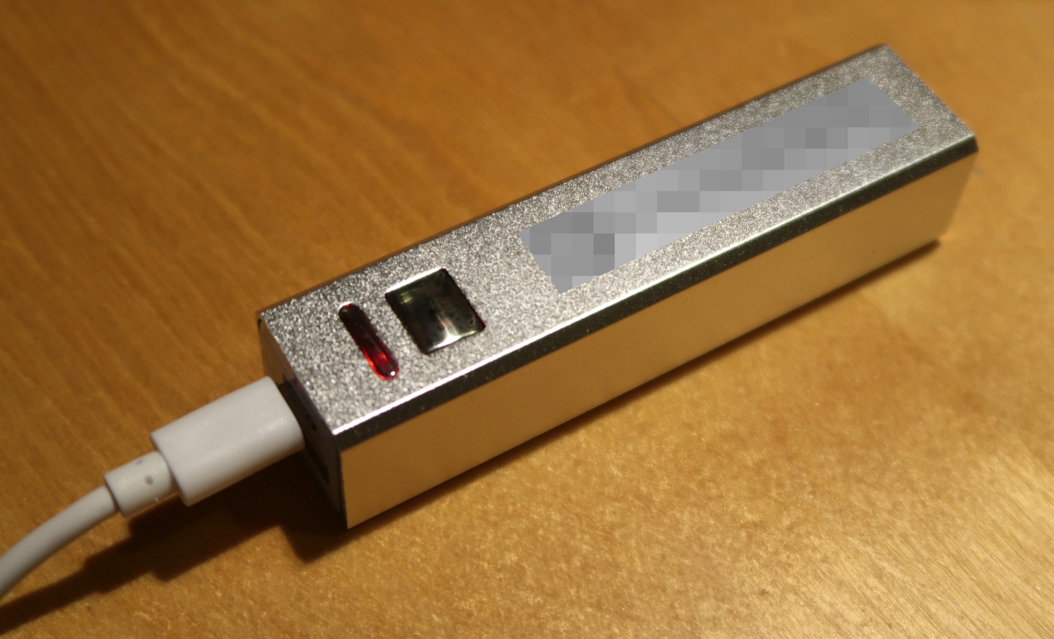
Figure 1: Power bank under test with a tastefully pixelated logo of the company I got this gadget from

Experimental part
The power bank was fully charged and then a 10cm cable with stripped wires on one end and a USB-A connector on the other was used to connect the power bank to a MightyWatt R3 electronic load (24 A/3 A, 30 V/5.5 V range).
A constant current of 0.5 A was drawn from the power bank until it switched itself off. Charge was calculated by integrating the measured current over time and total delivered energy was calculated by integrating the product of measured current and voltage (i. e. power) over time. The voltage drop across the cable was compensated for by measuring the cable resistance and increasing the voltage used for calculation of power by the product of current and cable resistance.

Results and discussion
The voltage from the power bank varied between 4.85 V and 4.88 V, which means the regulator kept a very stable voltage throughout the discharge and provided voltage high enough to charge devices connected to the power bank.
The power bank shot itself down after 2 hours, 14 minutes and 45 seconds after delivering 5.33 Wh of energy and showing a useful capacity of 1.12 Ah at the output voltage, which corresponds to 1.48 Ah at the nominal 3.7 V of the internal battery, not including losses at the internal boost converter. The stated capacity was 2.2 Ah (Figure 2), which means the power bank failed to deliver what it promised and was only able to deliver about 67 % of the stated capacity. Using a ballpark figure of 90 % boost converter efficiency, the power bank delivered 75 % of the stated capacity. Considering the unit was brand new, it is a rip off.

Figure 2: Power bank specifications showing the rated capacity in wrong units (mA instead of mAh)

Conclusions
Cheap power bank failed to deliver what it promised on the packaging. You can expect about 2/3 of the stated capacity to be really available. That being said, it is actually usable if you take the stated capacity with a pinch of salt and you don't mind that the device does not have any indication of the remaining capacity.

Crappy USB cable under test

What is in this test (Introduction)

This is a test of power handling capability of a really cheap USB cable. How cheap? I don't know because I found this cable in my box of USB cables. I probably got this bundled with some device. What you will find inside this test? A (not so) shocking revelation that chinese manufacturers are able to make a cable with virtually no copper at all.

I wasn't really going to test the cable in the first place. I was actually going to test a cheap powerbank I got as a corporate gift. You know, one of those small powerbanks that have a single 18650 cell inside and a boost converter ending in a USB port. And for testing, I needed a cable so I could connect it to my MightyWatt R3 electronic load. So I cut the cable, saving only the USB-A connector end with a few centimetres of cable. Inside, I found four tiny conductors that had barely any metal in them.

How I tested the cable (Experimental part)

The USB-B connector was cut from the remaining part of the cable, which was subsequently used for the experiment. The length of the cable for experiment was measured using a tape measure. Both ends of the crappy cable under test (CCUT) were stripped and the foil and braided shielding was removed (Figure 1). Using the removed part with the USB-A connector, the power conductors were identified to be red (V_BUS) and grey (GND). These conductors were stripped to bare copper and twisted together at one end, forming a single conductor.

Figure 1: Crappy USB cable and its internal conductors. Red wire – V_BUS, gray wire – GND. Green and white wire – differential data pair.

A power bank was used as the power supply. A MightyWatt R3 electronic load (24A/3A, 30V/5.5V ranges) was used as the measurement device.

The positive terminal of the power bank was connected to one end of CCUT, the negative terminal was connected to negative (PWR-) terminal of the load. The other end of CCUT was connected to positive (PWR+) terminal of the load. The voltage-measuring (sense) terminals of the load were connected at the ends of CCUT to measure the voltage drop across it (Figure 2).

Figure 2: Measurement setup showing MightyWatt R3 electronic load, power bank and CCUT

A 30-second linear sweep from 0 to 0.5 A was applied by the load followed by 60-second constant current at 0.5 A. Voltage drop across CCUT was measured as well as the applied current. The resistance was calculated as a ratio of voltage drop and applied current at the beginning of the 60-second constant current phase. The ambient temperature was 22 °C. Approximate cable gauge was estimated from the experimental data using a table on Wikipedia.

 

So how bad was it? (Results and discussion)

Pretty bad…
The total resistance was 3.7 Ω and slowly increasing as the cable was heating up. The length of the cable was 1.55 m so back and forth 3.10 m. That means the specific resistance was a solid 1.19 Ω/m, which is horrible. The wire gauge was approximately 36 AWG and its cross-section around 0.0127 mm², which can be safely rounded to zero :-) If you really put 0.5 A through this cable, you would get 1.85 V drop, which would probably cause any device supplied from that cable not working.
On the bright side, MightyWatt R3 turned out to be great at such an experiment. The accuracy within 1 % was available when the current was a meager 1/180 of the used range (Figure 3).

Figure 3: Relative measurement error as a function of current range. Accuracy better than 1 % starts at approximately 1/180 of the current range. Heating causing the increased resistance is visible as the vertical slope at the right end of the curve.

 

The bottom line (Conclusions)

Crappy cables are crappy. And at the USB 2.0 maximum current may be totally unusable.
May this be a cautionary tale and also an inspiration how to use an electronic load to measure stuff!

MightyWatt R3 Resource Page

This page contains the most up-to-date resources for MightyWatt R3. 

 

If you are looking for resources for versions 2 to 2.5, click here.

 

Resources on GitHub.

 

Latest release and factory calibrations also available on Google Drive.

 

Please, contact me if you found a bug or have a software request.

Latest hardware revision: 3.1.0

Latest sketch (firmware) version: 3.1.7 (3.1.0 calibration)

Latest Windows control program version: 3.1.4.8

Application notes

Contains guides and ideas on how to extend the use of MightyWatt R3.

Arduino firmware

Main (firmware): This is the program that runs in Arduino. It is compatible with Arduino Uno and Zero (M0/M0 Pro) board.
Calibration sketch: Use this for manual calibration of MightyWatt R3 together with calibration aid. See the Detailed guide on how to perform calibration.

Calibration aid

Excel spreadsheet: Calculates the calibration values from values obtained using the Calibration sketch. Replace default values in Configuration.h of the main firmware.

Calibrations

This folder contains factory calibration files for units sold through Tindie.

Case

SVG drawing: Contains drawings of the layers. See the folder readme for the number of layers needed.

Guides

Detailed guide: All you need to know for calibrating and running MightyWatt R3.
Case assembly instructions: If you have the original acrylic layered case for MightyWatt R3 for Arduino Uno or Arduino Zero (M0/M0 Pro), these are the instructions on how to assemble it.
Communication protocol description: If you wish to use your own PC-side control program with the original firmware, this guide has information about the communication protocol which is used by MightyWatt R3.
Booster pack guide: A guide for the official Booster pack accessory. Increases the maximum power dissipation with a power resistor.

Schematic and BOM

Eagle source files for the PCB of MightyWatt R3.
PDF schematic also included for a quick reference without having to install Eagle.
PDF Bill of Materials.

Windows control program 

Complete C# project: A PC-side program that controls MightyWatt R3. Program has manual control, advanced measurement programs, data logging, graphs and statistics. The executable is located in C#/bin/Release/MightyWatt.exe

MightyWatt Revision 3: Brand New and Seriously Improved

I have developed a new version of MightyWatt, the R3! It looks almost the same on the outside but is very different on the inside. It addresses shortcomings of the revision 2 and adds some new functions. But first, what is MightyWatt R3 (skip to Hardware changes if you already know…):

MightyWatt R3 on an Arduino Uno board

MightyWatt R3 is a programmable electronic load. That means you can use it for testing batteries, power supplies, fuel cells, solar cells and other sources of electrical power. You can also make a programmable power supply from a fixed-voltage power supply and MightyWatt R3 and use it for example as an intelligent battery charger.

MightyWatt R3 is made as an Arduino shield. Simply put it on an Arduino, upload the control sketch, open Windows control program and you are ready to go. In its heart, MightyWatt R3 has a special FET designed for linear operation that acts as a programmable resistor. It is controlled by an analog feedback loop that is able to keep either constant current or constant voltage (constant power and resistance is kept by a software loop). The current or voltage is set using a DAC, the actual voltage and current is read by an ADC so MightyWatt R3 has an integrated ammeter and voltmeter, both of which have two ranges with very fast autoranging. For the voltage measurement to be as precise as possible, MightyWatt R3 offers 4-wire (Kelvin) measurement where voltage is sensed by a dedicated pair of connections. This removes the effect of cable resistance from the measured value. It is of course possible to measure the voltage at the input terminals too (2-wire measurement). The power is dissipated in a force-cooled heatsink that is able to, with its fan, dissipate up to 70 Watts continuously. Current range is up to 24A and voltage up to 30V. MightyWatt R3 is 100% open source – hardware, firmware, software – so you can make your own one. Or buy a ready-to-use unit on Tindie.

Hardware changes in Revision 3

 

Schematic of MightyWatt R3

Dedicated ADC

While the revision 2 used Arduino's internal ADC, the new version has a dedicated delta-sigma ADC. Either ADS1115 (16-bit) or ADS1015 (12-bit). This means that the measurements will be more precise, less noisy and the calibration will hold for a MightyWatt R3 as a unit, regardless of the control board (Arduino) used.
Both supported ADCs have internal programmable gain amplifier so their resolution is effectively 4 bits larger. However, since they use one half of their range (negative values are not used), one bit is unused so in the end they behave almost like 19-bit and 15-bit devices.
To complement the new ADCs, the DAC can also be a 16-bit AD5693RBRMZ or a 12-bit AD5691RBRMZ (same as in revision 2).

Two current ranges

Instead of the one current range of its predecessor, MightyWatt R3 has two, separated by a factor of 8. Thus, a 24A version will also have a 3A hardware range. This will enhance the resolution and precision making MightyWatt R3 very usable even at low currents. The current sense resistor will, apart from Vishay WSL3637, now support also Ohmite LVK24 and LVK12 footprints, suitable especially for low currents.

Improved linearity towards zero

Analog voltage and current measurement have an intentional offset so the rail-to-rail operational amplifiers will remain in their linear range. Since both voltage and current are measured differentially against that offset, the measurement is even more precise than the single-ended measurement in revision 2 and the offset is of course completely eliminated from the result.

Better op-amps

The standard op-amps now include: OPA365 for the voltmeter and OPA197 as the FET gate driver. This is a definite improvement over the TLC2272/LMC6482 op-amp used in revision 2 both in terms of linearity and stability.

More stable gate driving circuit

More stabilization was added to the gate driver so the load is now very stable even with power supplies that have their own feedback for current and/or voltage. The compensation network is different for constant current and constant voltage mode and is automatically selected by the load.

More input protection

There is never too much protection so there are three new transient voltage suppressors – two on the voltmeter and one to protect the gate of the transistor.

Higher input impedance for the voltmeter

The standard resistors on the input are 1MΩ, three times the value of the revision 2 resistors. The burden on the device under test will be lower and the measurement more accurate, especially at low currents.

Switchable fan

The fan can be turned off when the load is small. MightyWatt R3 can dissipate about 10 W without the fan running so for low-power measurements, the fan can be turned off. The firmware will manage automatic turn on when the temperature or power dissipation increases above set threshold.

LED

LED is connected to PWM output from Arduino so its brightness can be controlled. Since it has a dedicated transistor now, it has an increased maximum brightness.

Firmware

Not only the hardware has changed. The firmware is now structured to several modules, each performing a dedicated task. It is more readable but also more complex because it has more functions. Some of the highlights:

• The communication now uses CRC checking of data integrity.
• The ADC control module performs filtering using a triangular weighted moving average filter to provide a smoother yet quick response.
• The main loop makes about 3000 turns per second on Arduino Uno (ATmega328P) and 150 complete measurements (V + I + temperature) per second.
• The software modes (constant power, constant resistance, constant software-controlled voltage and maximum power point tracker) have been reworked to settle faster.
• Firmware will allow short-term overload on voltage, current and power so quick transients will not abort the measurement…
• …but the protection logic will disconnect MightyWatt R3 within 10 ms from the time the power exceeded DC safe operating area of the transistor.
• Calibration sketch has been reworked too and is more automated and informative.

Windows application

And the changes also reflect in the Windows control application. Although most of the improvements lead to both a better accuracy and precision, something the control application has nothing to do with, user can now play with LED and fan rules and enable/disable the smoothing filter.

The LED and fan rules work like this: LED will light depending on some pre-defined conditions which can be combined. For example, it can light when the current is over 10% of the range or the temperature is above 50 °C.

The fan can automatically turn off with two settings that differ by what they will allow – either put emphasis on cooling (stricter rules) or emphasis on fan noise, meaning turning the fan off as often as possible (relaxed rules). The logic will still turn the fan on if the power or temperature is too high. It can, of course, be always turned on, which is the default setting.

Windows application now supports graphs using gnuplot and statistics so you can see how your measurement is progressing in real-time.

So all and all, improvements everywhere. It has still the same principle, but it just got way better! Get your MightyWatt R3 on Tindie or make your own one. MightyWatt R3 remains open-source. That hasn't changed and never will.

Resistor blackjack – the ultimate party game for nerds

Resistor blackjack is like regular blackjack but better! Your goal is to assemble a single resistance from several resistors that is as close to 21k while not being over.

Unlike regular blackjack, the resistors can be combined in series and in parallel, giving the game a whole new dimension. Plus, resistors have tolerances so achieving a mathematical 21k doesn't guarantee a win.

The deck

The deck resembles card deck except for the ace which has to be a fixed 11k.

For 4 players, you will need the following values:

2× 2k2

2× 3k3

2× 4k7

2× 5k6

2× 6k8

2× 7k5

2× 8k2

2× 9k1

8× 10k

2× 11k

Put all the resistors in a box and shuffle.

Player's equipment

Each player should be given an empty breadboard, resistor color code chart (maybe, if you want to be nice) and access to jumper wires.

Decide whether to allow calculators. Computing reciprocal values when resistors are combined in parallel can be tedious.

Dealer's equipment

Box with the deck.

Ohmmeter (multimeter).

Another box with: 5× 100k, 5×330k, 5×470k. 

A separate larger breadboard as the scoreboard.

 

Rules

Start the round by giving each player two random resistors. During the round, each player can ask for up to 4 more resistors (total of 6) but they have to use all of them and assemble them so they form a single resistance. Shorting a resistor is not allowed.

At the end of the round, dealer measures each player's assembled resistance. Who is the closest to 21k without being over wins and draws one resistor from the second box. The resistors which players win are connected in series on a separate breadboard (scoreboard) and who is the first to have over one million ohms wins the entire game!

Rule extension: 20k trimmer.

Before a round begins, dealer can ask a trivia question. The player who has a correct answer (is first or is the closest if the answer is a number) is given a 20k trimmer which he/she can but does not have to use in the following round. The trimmer is returned to the dealer after the round ends.

Hameg HM8118 LCR bridge

tl;dr: I made a control program for Hameg HM8118 LCR bridge. You can get it here: https://github.com/kaktus85/Hameg8118

Controlling Rohde & Schwarz Hameg 8118 LCR Bridge/Meter from PC

Introduction 

There's a lot of LCR bridges on the market from simple fixed-frequency el cheapo meters made in country where pandas kiss good night to high end thousands of dollars meters made in… well, the very same place.

Somewhere in the middle lies Hameg HM8118 LCR bridge from Rohde & Schwarz for about 2300 USD. While the less advanced models only have a couple of frequencies at best, this baby has 69 of them. That makes it suitable for measuring a frequency sweep and then fitting the data to a more complicated equivalent circuit than the two-component model you can use for a single frequency. The frequency range is 20 Hz to 200 kHz and the device has specified accuracy to 100 kHz so the frequencies between 100 kHz and 200 kHz are more of a "bonus". But that does not mean they are completely useless. Just that you can't expect them to be super-accurate.

Hameg HM8118

Operating principle

So, how does it work? Normally, the bridge measures the voltage and current through the device under test (DUT), which is typically a resistor, capacitor or inductor. Besides amplitudes, it also measures the phase and from the ratio of amplitudes of voltage and current and the phase difference, it then calculates the impedance. Either as magnitude-phase or resistance-reactance. It is just a different representation of the same quantity. Then, it can apply the knowledge of impedance together with the frequency on a simple two-component model such as a combination of resistor and capacitor or resistor and inductor. Plus, these components can be connected in series or in parallel. That is all math. The device calculates what would be the values of the resistor and capacitor/inductor if they've been connected in series or in parallel and the whole ciruit had the measured impedance at the set frequency. 

But as you only measure two quantities (voltage and current), you can only calculate two unknowns. If the circuit is more complicated, you need measurements at more frequencies. Preferably, you measure all the 69 available frequencies and then fit the experimental data to the equivalent circuit. Not a trivial task to do but possible.

This is the basic operating principle of this LCR bridge. It is a nice unit that, sadly, does not come with a desktop software so you have to rely on the front panel display and buttons which make complicated measurements tedious. Yet, you can connect the device via USB and switch it to a virtual COM (serial) port. Then send commands and read measured values.

Controlling from PC

I have used the serial port feature to create a simple control program in C# (.NET 4.6). It should work on any computer running Vista or higher. It is open source and released under GPL v.3. The project, which also contains the only executable file you need (Hameg8118.exe) is available on my GitHub account.

Push it to the limit – measure the true junction temperature to get the most out of MightyWatt

Spoilers!

If you just want to know if you can overload your MightyWatt, the answer is yes. You can run it at 75 W constantly and at about 85 W for short periods.

End of spoilers 

Fig. 1: Experimental setup for measuring forward voltage drop of a FET body diode.

Introduction

If you want to run a FET at high temperature, which is typical in electronic load applications, it is important not to exceed the maximum junction temperature. In my MightyWatt electronic load, I use IXTH75N10L2 as the main transistor and its maximum allowed junction temperature is 150 °C.

It is not easy to measure the junction temperature without actually having a sensor at the junction. Thermal camera, thermistors and other sensors will always measure less because there will be a temperature gradient betwen the case and the junction. At 70 W, the temperature of the copper tab directly attached to the die can be 20 °C less than the silicon temperature!

Luckily, there is a way of measuring the junction temperature. Sadly, it cannot be done while the load is operating… Because the temperature sensor is the intrinsic body diode of the FET itself. Its temperature coefficient can be measured in laboratory conditions and then its temperature can be correlated to some other temperature sensor, attached to the body of the transistor. In case of MightyWatt, that is a tiny 0402 thermistor placed beneath the transistor.

Experimental setup, results and discussion (don't mix this in a paper)

Measurement of the diode temperature coefficient

I have first measured the intrinsic body diode forward drop (V_SD) of 10 samples of IXTH75N10L2 at room temperature (about 24 °C) at 1 mA using Keysight 34461A bench-top digital multimeter. Interestingly, they were all the same, at 522 mV. That's good! Seems like the process variation is not very high.

Then, one sample from these 10 was randomly selected and fitted with silicone elastomer insulated cables to the drain and source.

The transistor was then immersed in an oil bath (edible rapeseed oil actually) in a borosilicate beaker with a magnetic stir bar and put on a heated magnetic stirrer (IKA C-MAG HS7) (Fig. 1, 2). The temperature sensor from the stirrer was Kapton-taped to the metal tab of the transistor.

Fig. 2: Transistor in an oil bath with two temperature probes: One from the magnetic stirrer/hotplate and a second, external one for verification.

Then, the bath was heated to 60, 70, 80, 90, 100, 110, 120 and 130 °C and when the temperature stabilized, a few seconds worth of experimental values were averaged to get the V_SD. The multimeter sampled at about 1000 samples per second.

The V_SD turned out to be linearly dependent on the temperature with a slope of -2.454 mV/K (Fig. 3).

Fig. 3: Temperature dependence of V_SD and ideality factor n (which is only discussed in the "extra math" section so pretend you can't see it).

Measurement of the diode V_SD in MightyWatt

First, I soldered wires to the drain and source of one standard MightyWatt's main transistor. The source was at the common ground potential. Because measuring V_SD means connecting the polarity in opposite, the drain was connected to a SPDT relay. The normally closed lead was connected to multimeter negative terminal (diode cathode) via a 0.15-Ohm current sense resistor while the normally open lead was connected to power supply positive terminal.

Triggering of the measurement was done using a comparator circuit, which was driving one transistor that switched the relay and another transistor which triggered the multimeter. When there was current flowing through the load, the comparator would switch the relay to connect the power supply. When the current was interrupted, the relay switched to measure the V_SD (Fig. 4). The propagation delay between the current interrupt and the actual trigger signal was measured using an oscilloscope (Rigol DS1052E).

Fig. 4: Schematic of the connections for the in-system measurement of V_SD.

The load was let to dissipate 75.9 W at 3.004 A and I waited until the temperature reported by a thermistor placed beneath the transistor was stable. This took about 10 minutes from ambient temperature. Then, the current was interrupted by physically removing USB cable that powered MightyWatt, immediately interrupting current flow. At that point, the relay switched and multimeter began to measure 2000 samples at about 1000 samples per second. I am only showing the first 500 ms, since the rest was a monotonic increase.

The V_SD quickly increased upon interrupting the current. The trigger propagation delay was about 0.2 ms and thus negligible. There was an 80-ms delay starting from the current interrupt before the sampled data stabilized. The V_SD had to be extrapolated from the recorded data to the point where the current was actually interrupted. I used only a phenomenological 5^th order polynomial to extrapolate to the beginning (Fig. 5). Thermal fluxes are complicated in such setup…

Fig. 5: V_SD development with time right after the current was interrupted. First 80 ms had to be extrapolated.

So the V_SD was about 260 mV when the current was interrupted, which means the junction temperature was about 132 °C, well below the maximum. By the way, the thermistor reported 101 °C temperature. The ambient temperature was 26 °C. 

We can calculate the thermal resistance of the system now: (132 - 26) / 75.9 = 1.4 K/W. While the thermistor thinks it is (101 - 26) / 75.9 = 1 K/W. We should therefore calculate the junction temperature (Tj) from thermistor temperature (Tth) and ambient temperature (Tamb) as Tj = (Tth - Tamb) / 1 × 1.4 + Tamb.

Assuming Tamb = 25 °C and Tj = 150 °C, the thermistor will be reporting about 114 °C at this maximum. MightyWatt will report overheat above 110 °C, which seems to be a correct threshold to allow some leeway.

The maximum dissipated power is then (150 - 25) / 1.4 = 89 W. And at rated 70 W, the junction temperature is about 70 × 1.4 + 25 = 123 °C. But there is one catch: The Arctic Silver AS5 thermal paste (which I use) is rated 130 °C continuously (180 °C for short periods of time). The temperature at the thermal paste is unknown because datasheet only quotes maximum junction-to-case thermal resistance. Using the maximum value, the case temperature at Tj = 150 °C will not be less than 122 °C. But probably it will be higher, possibly exceeding the long-term rating of the thermal paste. So to be perfectly safe, let's assume the Tj to be 130 °C maximum. At this temperature (and 25 °C ambient), the maximum continuous power dissipation is (130 - 25) / 1.4 = 75 W. 

We should leave some safety margin because the extrapolation might not have been very precise and the Tj could have been higher. But advertising MightyWatt as a 70 W load seems to be honest, if a little conservative. And don't worry overloading it for extra 15 W for short experiments. You will have to change the maximum power in the sketch though.

That's all folks! But if you're interested in some more math, then please, continue reading…

---

Digging deeper

Calculation of V_SD

Besides direct measurement, the V_SD can be calculated using Shockley diode equation (1), where I is the diode current (1 mA in this case), I_S is the reverse bias saturation current, n is the ideality factor, typically between 1 and 2, and V_T is the thermal voltage equal to kT/q, where k is the Boltzmann constant, T is the thermodynamic temperature and q is the elementary charge.

(1)     I = I_S[exp(V_SD/n/V_T) - 1]

I_S is temperature dependent and is approximately equal to (2), where E_g is the bandgap energy.

(2)     I_S = T³exp(-E_g/k/T) 

The bandgap energy also depends on temperature and can be calculated from (3), with experimentally determined parameters E_g(0) = 1.166 eV, α = 4.77·10^-4 eV/K and β = 636 K.

(3)     E_g(T) = E_g(0) - αT² / (T + β)

Combining equations 1, 2 and 3 with the experimental data permits the calculation of the only remaining unknown – the ideality factor n – which was calculated to be between 1.061 and 1.175 for the temperature from 60 to 130 °C (Fig. 3).

The value of n indicates that the current was limited mainly by the recombination of minority carriers in the neutral region.

Junction temperature under load

Thermal fluxes in systems like transistors on an active heatsink are complicated. The heat emerges from a relatively small region made of silicon and is then preferentially conducted via copper tab to the back of the transistor case where a heatsink is attached. The silicon content is very low compared to the lead frame and encapsulant, which contribute to almost the entire heat capacity of the device.

IXYS does not publish information about the material composition of the transistor but a similarity can be assumed with other parts in the same package. International Rectifier publishes Bill of Materials for TO-247 packaged transistors. The main mass (66.2 %) of the transistor is the copper lead frame. The other significant contribution is the epoxy resin, that is composed mainly of a filler – SiO₂. These two materials account for over 90 % of the overall mass. The silicon content is a meager 0.6 %. The total weight of the transistor, as reported by International Rectifier, is 5.6 g. The IXYS IXTH75N10L2 was somewhat heavier at 6.4 g.

This permits us to calculate the approximate heat capacity of such transistor. The specific heat capacity at 127 °C of Cu, SiO₂ and Si is 398.6, 889.2 and 788.3 J/kg/K respectively. Assuming the balance to 100 % has the same average heat capacity as the two main components, the overall heat capacity of the International Rectifier transistor is approximately (398.6 × 0.003719 + 889.2 × 0.001411)/0.913 = 3.00 J. Scaling this to the IXYS transistor, the heat capacity could be about 3.00 × 6.4/5.6 = 3.43 J.

Assuming the transistor is evenly heated and thermally conductive, the 80 ms delay at 75.9 W of cooled power would cool it by 1.8 K. However, such assumption is never true because the materials have different thermal conductivity and the heat distribution is uneven, with the maximum at the junction. Besides that, the silicon part has very low heat capacity because it is very small and the thermal path is mainly through the copper to the heatsink. There is a large temperature gradient from the junction to case at 75.9 W. According to the datasheet, the junction-to-case thermal resistance is up to 0.31 K/W, which creates a gradient of 23.5 K at 75.9 W. The extrapolation of junction temperature, even to a time only 80 ms before experimental points, is not trivial and in this study was done by simply fitting the V_SD vs. temperature curve with a 5^th order polynomial that accurately tracked the experimental data (Fig. 5).

Well, if you read all of this, you really pushed it to the limit. Go ahead, you deserve it!

Virtual ground

Introduction

Bipolar is not only a disorder but also a requirement for power supply for some devices. While most electronics is OK with a simple plus and minus, some will also require a mid-point, often called ground. It does not have to be connected to a real Earth ground and sometimes that is not even possible (think satellites).

The problem is that many laboratory power supplies do not have this midpoint, though they frequently offer ground connection. But that can only be tied to plus or minus, no real midpoint is typically available on them. That's where a virtual ground comes to save the day. Virtual ground, also called "rail-splitter", is a device that creates a midpoint, whose voltage is (plus + minus)/2 and is capable of both sinking and sourcing current. There are two basic approaches to get virtual ground: Either from a switching regulator or from a linear one. The former is more efficient and the latter is easier to build and offers less noise, albeit at the cost of wasting half the power.

For projects that do not require high power, a linear virtual ground is appropriate. I am presenting a circuit and a board that I use personally. It is a third iteration of my original design using a power op-amp and a simple resistor divider.

The construction

My virtual ground is not cheap, it uses quality components and you may find a cheaper alternative. But this design is robust, simple and powerful. The printed circuit board itself is around 20 USD at OSH Park.

Top of the PCB

Bottom of the PCB

The unipolar power enters through an universal screw clamp terminal (CON1), the positive rail passes through a 3A resettable fuse F1 (PTC). Voltage spikes are quelled by a bipolar (can be unipolar too) transient suppressor diode D1. The positive rail then passes through reversed P-FET transistor Q1 that protects the circuit from reverse polarity. A suitable part for Q1 would be Vishay SUD50P06-15, a cheaper alternative Infineon SPD18P06P G might work too. Gate voltage is regulated by Zener diode D2 and current-limiting resistor R1. The gate voltage must stay below what is in the datasheet (typically 20 V) so choose the Zener voltage few volts below the FET's maximum (see my earlier blogpost about reverse polarity protection). The rail then continues from Q1 to three bypass capacitors for the main op-amp. C1 is an aluminium electrolytic capacitor, C2 a large ceramic capacitor and C4 is not shown because it is supposed to be soldered directly between pin 4 and 5 of the op-amp. Use 0603 package and 100nF/100V with X7R dielectric.

Schematic of the virtual ground (click for full resolution)

The voltage from the input terminals is divided by two thin-film precision resistors. Use at least 56k because if the polarity is reversed, some current will go through these resistors and the ESD diodes of the op-amp. Its value should be small (like 1 mA). The output of the resistor divider is one half of the input voltage, this, after being buffered, will be the virtual ground voltage. The output from this resistor divider is stabilized using capacitor C3.

The heart of the virtual ground is OPA548 – a high-end power operational amplifier from Texas Instruments (IC1). It is capable of continuously outputting 3 A. Its input voltage must be between 8 and 60 V so the virtual ground will be 4 to 30 V above the negative power supply. Since this is a linear virtual ground, the op-amp must be attached to a heatsink. With Fischer Elektronik SK 129 63,5 STS, the thermal resistance of the system should be around 5 K/W so the virtual ground will be capable of dissipating approximately 20 W. But I haven't tested it at this power dissipation.

The output of IC1 is buffered by two identical aluminium electrolytic capacitors – C6 and C7 – before entering the output banana receptacle. A snubber circuit aimed against oscillations is formed from a series combination of resistor R4 and capacitor C5. Two reverse-biased silicon diodes (D3, D4) protect the output of the IC1 against voltage spikes that often occur from inductive loads. A suitable diodes are MUR410 from ON Semiconductor. Fast recovery is a key factor here.

Finally, there is a green LED (LED1) with series resistor R5 indicating that the output is on.

How to calculate power dissipation

It is simple: the virtual ground must drop one half of the input voltage, so the power dissipation is the input voltage, divided by two and multiplied by the current. Or – the output voltage in respect to the negative input voltage, multiplied by the current.

Conclusion

The idea is simple, the execution likewise. Input protection, resistor divider and a unity-gain power amplifier with output protection. If you're going to build this, don't forget a good thermal grease between the heatsink and op-amp and maybe add some rubber feet to the bottom of the board.

You may want to consider thicker copper layer, such as 2 oz/sqft instead of the standard 1 oz/sqft.

Eagle project can be found on my Google Drive here and on GitHub.

USBuddy

Do you sometimes develop with USB? I do. So I need to access data lines, bus voltage and I'd like to easily monitor the current too. I made myself a small companion (43.5 mm × 22.5 mm, 9.5 g) to do that. Just a simple breakout board with one connector in and one out. And a little extra to make things easier. I call it USBuddy.

USBuddy between host and device.

It has one pin header to break out all the lines plus one LED to indicate that the USB is on. And the current measurement system: It is a very simple system, just a current shunt resistor and a current shunt amplifier. I chose INA199B1 with 50 gain which consumes less than 100 µA. This allowed me to use a very small current shunt, just 20 mΩ. This means that at 0.5 A, I will be losing only 10 mV. And it also means that the output will be a convenient ratio of 1 mV = 1 mA. The current shunt has 4-wire (Kelvin) connection for more precise measurement.

But why stop here? Often, USB is used for charging at larger currents. The design allows for up to 4 A and 24 V. While putting more than 5 V on USB is typically not a good idea, the USBuddy is designed to handle that just well.

USBuddy schematic

If you think this project can help you, you will find all the design files on my Google Drive and on GitHub.

MightyWatt: How to increase the maximum power dissipation

Sometimes, you just need a bit more power than MightyWatt can dissipate. There is one trick that can easily increase the maximum dissipation. If you test batteries, they aren't typically discharged to zero voltage. This can be exploited: If you put a power resistor in series with the load, it will take over some of the heat that will be dissipated during testing, leaving a smaller portion to the load.

Let's make an example: Suppose you have a lead-acid battery that you want to discharge at 8 A. The battery goes from 14 V to 9.5 V. That would mean 112 to 76 W, well beyond the maximum for standard MightyWatt. However, if you put a 1 Ohm power resistor (properly rated) in series with the battery, it will dissipate 64 W while producing an 8 V drop in voltage. The load will only have to dissipate the rest: 48 to 12 W. Thanks to the differential voltmeter, you will always have the accurate battery voltage when using 4-wire mode as well as the total power of the device under test.

Schematic of connection with power resistor

A suitable power resistor would be for example this one from Vishay: HL10006Z1R000JJ or this one from Multicomp: MC14668. The first one is 7 USD on Mouser, the second one 9 USD on Farnell/Newark. That's a pretty cheap extension of the power dissipation!

Typical shape of a suitable power resistor

Now, there are some important points about this approach:

• Because the power dissipation is calculated simply as the product of voltage and current, you will have to tell MightyWatt that you are using a series resistance so it won't show overload. In the Windows control program, select Advanced => Series resistance and type the value of the external power resistor in the pop-up window. The load will automatically keep track of the true dissipated power in 4-wire mode. This value only affects the thermal management, nothing else. But be careful, if you put wrong value or you remove the power resistor later, it may lead to a damage of the load.
• This only works as long as the power difference between charged and discharged state (start - end) is not higher than the MightyWatt rating. It is great for batteries but if you have to go all the way down to zero with the voltage, you will have to split the experiment (voltage ranges) into two or more parts.
• The temperature coefficient and precision of the power resistor do not matter much. The voltage is measured directly on the device under test and current measurement is not affected either. Don't waste money on high-end power resistors.
• There are power resistors in aluminium heatsinks that look like the one below. These have to be mounted on a large heatsink to dissipate the rated power. See their datasheet. These resistors cannot dissipate the rated power only with the small heatsink that is around them. 
 

Power resistor that has to be mounted on additional heatsink

Current accuracy of MightyWatt

People sometimes ask me how accurate is MightyWatt. I made a lot of tests during the development stage but how does a production unit (revision 2.5) perform? When I got my new Keysight 34461A, I thought it is about time to find out…

If you want raw data, click here to get the full report (Excel)

MightyWatt with Arduino Uno

While MightyWatt has its own 12-bit DAC, it relies on the ADC of the control board, which is typically Arduino Uno. The ATmega 328P in Uno has a 10-bit ADC. The sketch oversamples it to 12 bits.

The setup was:

• One standard MightyWatt 30V/10A/70W with standard terminals
• Original Arduino Uno running firmware (sketch) 2.5.1
• Linear laboratory power supply PSD30/3C, 30V/3A
• Keysight 34461A multimeter on autorange, current measured in 3A terminals, 10 PLC integration

First, MightyWatt was calibrated according to the manual from 0.1 to 3A with 5 calibration points. Since I only had 3A power supply, the calibration range was up to that current.

Calibration constants let us calculate the current resolution offered by DAC and ADC. DAC and oversampled ADC had one LSB equal to 2.56 mA. Physically, the ADC LSB was 10.23 mA before oversampling.

Then, I set a specific current via the Windows control program and noted the current that was measured by ADC and the true current from 34461A.

MightyWatt set I, A	MightyWatt measured I, A	External ammeter I, A
0.1	0.101	0.0982
0.25	0.255	0.2494
0.5	0.500	0.4980
1	1.001	1.0001
1.5	1.498	1.4997
2	1.994	1.9992
2.5	2.495	2.4985
3	2.997	3.0080

So, what these numbers tell us? Let's calculate the relative errors from the true value in percents and absolute errors in LSBs. Because the ADC was oversampled, there are both physical (p) and oversampled (o) LSBs in the table.

Set I (DAC) error	Measured I (ADC) error
1.83 % / 0.70 LSB	2.85 % / 0.27 LSBp / 1.09 LSBo
0.24 % / 0.23 LSB	2.25 % / 0.55 LSBp / 2.19 LSBo
0.40 % / 0.78 LSB	0.40 % / 0.20 LSBp / 0.78 LSBo
-0.01 % / -0.04 LSB	0.09 % / 0.09 LSBp / 0.35 LSBo
0.02 % / 0.12 LSB	-0.11 % / -0.17 LSBp / -0.66 LSBo
0.04 % / 0.31 LSB	-0.26 % / -0.51 LSBp / -2.03 LSBo
0.06 % / 0.59 LSB	-0.14 % / -0.34 LSBp / -1.37 LSBo
0.08 % / 0.98 LSB	-0.02 % / -0.05 LSBp / -0.20 LSBo

One thing is immediately obvious, the DAC performed better than the ADC. This is, however, no surprise. The DAC is a standalone chip of good quality with 12 bits of resolution while the ADC is integrated in a microprocessor with 10 bits of resolution. It was an unfair match to begin with.

However, the overall accuracy was pretty good, DAC did not exceed 1 LSB error and ADC too if you count the physical LSB as the LSB. It is also worth recommending not to operate the load below 1 % of the range. The relative error there was almost 2 % of set current and 3 % of measured current. Above this threshold, the accuracy quickly improved.

The root mean square of absolute error was 0.57 LSB for DAC and 1.29 LSB for oversampled ADC. That means the DAC was about 2.3 times more accurate than the oversampled ADC.

If you recalculate the relative accuracy to the full scale (10.5 A in real), the worst error was 0.024 % of full range for set current and 0.053 % of full range for measured current.

So, would it improve if we used Arduino Due?

MightyWatt with Arduino Due

Due has 12bit ADC already and with some averaging, we can get even better accuracy from it.

Besides the Due itself, the setup was the same as with Uno.

Again, MightyWatt was calibrated according to the manual from 0.1 to 3A with 5 calibration points. Since I only had 3A power supply, the calibration range was up to that current.

The LSB for ADC was 2.55 mA while for the ADC 2.56 mA, practically the same.

MightyWatt set I, A	MightyWatt measured I, A	External ammeter I, A
0.1	0.098	0.09818
0.25	0.249	0.2494
0.5	0.499	0.4979
1	1.001	1.00006
1.5	1.501	1.4997
2	2.001	1.9992
2.5	2.498	2.4986
3	2.998	2.9974

Comparing this with the Uno measurement, the true current was pretty much the same with the same set values. That was because the DAC did not change and it performed similar to the first experiment.

Set I (DAC) error	Measured I (ADC) error
1.85 % / 0.71 LSB	-0.18 % / -0.07 LSB
0.24 % / 0.23 LSB	-0.16 % / -0.16 LSB
0.42 % / 0.82 LSB	0.22 % / 0.43 LSB
-0.01 % / -0.02 LSB	0.09 % / 0.37 LSB
0.02 % / 0.12 LSB	0.09 % / 0.51 LSB
0.04 % / 0.31 LSB	0.09 % / 0.71 LSB
0.06 % / 0.55 LSB	-0.02 % / -0.24 LSB
0.09 % / 1.01 LSB	0.02 % / 0.24 LSB

The ADC in Due is vastly superior to the one in Uno. With 16 sample averaging, as defined in the sketch, it is even better than the DAC. The root mean square error was 0.58 LSB for DAC and only 0.39 LSB for the averaged ADC. The choice for high precision measurements is Due.

The worst accuracy relative to full scale (10.5 A) was for both ADC and DAC 0.025 %.

Temperature coefficient

 

While the measurements were accurate at ambient temperature, things can change when they get hot. And electronic load is designed to be operated at high temperatures. I set 3 A and 23.3 V to get 70 watts of dissipated power, the maximum continous rating for the standard MightyWatt. The time constant for the whole load is about one minute so after 10 minutes, the load is in thermal equilibrium. The change in temperature was from 21 to 88 °C, as reported by the thermistor underneath the MOSFET.

At 21 °C, the current, as read by the 34461A, was 2.9975 A and at 88 °C it was 3.0080 A. Recalculating this to the temperature coefficient, its value was 50.0 ppm / W, or 52.3 ppm / °C. Interestingly, the temperature coefficient of the current sense resistor is 50 ppm / °C according to the datasheet.

Noise and stability

 

Not only one-shot accuracy is interesting, the noise in the measurement and its stability is important too. I tested the stability at 1 A set current and acquired 600 samples with the 34461A. The statistics is below:

Average current	1.0003711 A
Standard deviation	0.0000132 A
Relative standard deviation	0.00132 %
Minimum value	1.000331 A
Maximum value	1.000416 A

MightyWatt was indeed exceptionally stable in the DC measurement. But what was the AC, or noise component of the signal? I set the load to measure AC current and the multimeter to acquire anything from 3 Hz to about 300 kHz, which is the upper range of the multimeter. The noise was then expressed as the AC/DC ratio.

MightyWatt set I, A	AC RMS I, A	AC/DC ratio
0.1	0.000235	0.24 %
0.5	0.00014	0.03 %
1	0.00063	0.06 %
3	0.00167	0.06 %

Noise was low and again, the best measurement was when the current was above 1 % of the range. Just a note: a certain amount of noise helps the ADC on Uno with oversampling. A perfectly clean signal cannot be oversampled…

Conclusion or How to make accurate measurements with MightyWatt

• Stay above 1 % of the current range.

• MightyWatt performs very well with Uno but if you are looking for the very best accuracy that is possible, use Arduino Due or similar board with good ADC.

• If you are making a lot of measurements at high power, consider calibrating the unit at the desired temperature. You can control voltage during current calibration and current during voltage calibration so it is possible to get a specific temperature. This will compensate for the temperature coefficient.

• The calibration is only as good as your reference is. The ammeter and voltmeter should be, ideally, 10 times as precise as the precision you want from MightyWatt.

• The internal reference voltage in the DAC can take some time to stabilize. It is a good practice to let the unit on for a couple of minutes before taking measurements. Most lab equipment accuracy is specified only after the unit has been turn on for a certain amount of time.

MightyWatt as a Li-Ion charger

Introduction

MightyWatt electronic load can be used not only to test how a battery is discharged but it can also be used to charge the battery. In conjunction with a fixed-voltage power supply like a wall wart, MightyWatt can be turned into a USB programmable Li-Ion charger with CC/CV mode.

 

Typically, a Li-Ion battery is first charged by a constant current. When a certain voltage is reached, for example 4.2 V, the charger then keeps the voltage constant until the current drops below some pre-defined threshold. Then the charging process is considered finished.

You can use the MightyWatt in conjunction with a cheap fixed-voltage power supply to create such charger. By connecting MightyWatt in series with the battery and power supply, it will be possible to control the current (and voltage) while measuring voltage at the battery terminals. This is possible thanks to the differential voltmeter whose inputs can be at different potential than the power terminals.

Setting it up

First, be sure that you have a firmware version at least 2.5.1 and Windows control program 1.2.2.0 or higher (get it here).

So, how to do it? First, make the connection (Figure 1): Connect the positive terminal of the battery to the positive terminal of your power supply. Connect the negative terminal of the battery to the positive power terminal (PWR+) of the MightyWatt. The negative power terminal (PWR-) is then connected to the power supply ground. This signal ground will be also the earth ground because the PWR- is connected to earth via USB.

Now, connect the positive sense terminal (SENS+) to the positive terminal of the battery and the negative sense terminal (SENS-) to the negative terminal of the battery. In this way, you will be able to measure the voltage of the battery while controlling the charging current.

Figure 1: Connection schematic to create a programmable CC/CV Li-Ion battery charger.

Let's set the control software correctly now (Figure 2). In this example, I will assume that the battery should be charged with 1 Amp to 4.2 V and then kept at 4.2 V until the current drops to 50 mA.

1. Safety first: Set up the watchdog. If anything goes wrong, the load will disconnect the battery. I have set the watchdog to stop if current exceeds 1.5 A.
2. Set the remote (4-wire) voltage sensing.
3. Define the constant current part of the charging process. I put 1 A for 3 hours (the time limit won't be reached so put something long here). Then define the skip conditon. That means this part of the charging will be terminated when the condition is met. I chose that exceeding 4.2 V will make the program go to the next step.
4. Define the constant voltage part. It is important to set "constant inverted phase voltage", I will talk about it later. In my example, I will keep 4.2 V for 3 hours (it will finish sooner so once again, put some long time here) and terminate this part when the current drops below 50 mA.
5. If you wish, set up logging and/or save the program items for future use.
6. Hit the Start button, you're ready to go!

Figure 2: Setting of a CC/CV mode for battery charger. Watchdog is enabled for safety.

What is the "constant inverted phase voltage" all about?

 

The second part of the charging process requires the voltage to be kept constant. However, it is not possible to directly use the hardware implemented constant voltage because it has an incorrect phase for this application. Normally, the constant voltage mode assumes that by increasing the current, the voltage will drop. This is normal behaviour of most sources. But look at this setup: increasing current to the battery will actually increase its voltage. It is the difference of power supply voltage and battery voltage that is in fact decreasing. But we want to measure (and control) the battery voltage, not the power supply that is actually loaded. 

So the feedback has to be modified to a system where increasing the current will increase the voltage. In other words, the transistor in MightyWatt must open when the voltage is too low and close when it is too high. This is not implemented in hardware so the firmware must be called to help. In the mode named "constant inverted phase voltage" the firmware (Arduino sketch) will internally switch the load to constant current mode and then increase it when the voltage is lower than the set voltage or decrease the current when the voltage is higher than the set value.

The bottom line

 

With the new firmware and software, you can turn your MightyWatt (+ cheap power supply) into a great USB programmable Li-Ion battery charger! Use the special "inverted phase voltage" mode to keep the voltage constant in this setup. If you don't have the latest firmware and software, download it from the resource page. Don't forget to copy your calibration values.

Building a 100 mA transimpedance amplifier

Introduction

A while ago, I wrote about zero resistance ammeter. The more common name for it is transimpedance amplifier. It is a device that converts current to voltage. So an ammeter really. But unlike the ordinary ammeter, transimpedance amplifier (TIA) has zero voltage drop across its terminals. To achieve that, it has to be an active device. The most simple form comprises of an op-amp in inverting configuration with a single resistor, RF, that determines the transimpedance gain. In reality, there has to be an additional capacitor, CF, to compensate for the op-amps input capacitance [Figure 1]. The output voltage is then V = -RF·I.
An excellent overview on this topic from Robert A. Pease can be found here: http://electronicdesign.com/analog/whats-all-transimpedance-amplifier-stuff-anyhow-part-1.

Figure 1: The principle of transimpedance amplifier.

The big advantage of TIA is that is has zero voltage drop on its terminals so it does not affect the circuit being measured – unlike a regular multimeter. Also, regular multimeters tend to be much less precise on current measurements than on voltage measurements. Using a precision current to voltage converter, you can increase the precision of measurement and not influence the measured circuit at the same time!

When one range is not enough

If you need more gains (ranges), then you can place a switch in series with the resistors. It is a good idea to have a make-before-break (shorting) switch so you don't interrupt the flow of current during switching. The switch, however, adds uncompensated capacitance and series resistance. This limits the use of semiconductor switches because their capacitance is typically higher than the capacitance of mechanical and electromechanical (relay) switches. Switch resistance will produce a measurement error which increases when the value of gain resistor decreases. It is possible to use a double throw switch and use the second part to sense the voltage drop before the current enters the first part of the switch.

Powering from a single supply

To have a bipolar ammeter on single supply, you will need another op-amp for biasing. This op-amp needs to be as fast and as powerful as the first one. Remember, the op-amps will be sourcing/sinking the same current you are measuring.

The prototype

 

The design idea

My design [Figure 2, 3] uses two OPA567 power op-amps in non-inverting configuration supplied from a single cell li-ion battery (RCR123A). One of the op-amps is held at bias voltage of 1.25 V (from a series voltage reference). The second is controlled by OPA320 in such a way that its voltage creates zero potential difference between the sense terminals. The reason for using OPA320 is that its input offset voltage is very low. Both OPA567s are used only for their high current capabilities. This configuration also enables easy remote (4-wire) sensing which elliminates the input cable resistance [Figure 4].

The current passes through precision (0.1%) resistors, the switch and two protecting PTCs. The voltage drop across the precision resistors is multiplied by two using an instrumentation amplifier INA333 referenced to the 1.25 V node. This amplifier isolates the voltage output so any loading of the output terminals does not affect the TIA's operation. The output voltage range is ±1 V so the voltage drop across the precision resistors is 0.5 V maximum. The remaining 0.75 V can be (although not entirely because the OPA567 cannot swing to exactly zero) sacrificed on other resistances, particularly the two PTC protection fuses and cables that will connect the TIA to its source.

Figure 2: Complete schematic of my transimpedance amplifier.

Figure 3: Finished prototype. The range is switched to 1 V = 1 mA. Green LED on the left indicates battery OK. Red LED on the right would indicated an overload.

Figure 4: Testing the input offset voltage. At 102.9 mA (range set at 1 V = 100 mA), the input terminals were 30 µV apart.

Safety and monitoring

Output is ESD protected by high-speed TPD2E001 diode array and 100R series resistors. Inputs are protected by series resistors (sensing) and PTCs (power). Battery input is reverse-polarity protected and also has a PTC and a TVS.

A microprocessor (ATTINY24A) monitors the battery voltage, output voltage of the instrumentation amplifier and output voltages of both power op-amps. Firmware controls whether the battery is OK and the output voltages stay in the device limits so there will be no clipping of the signal. Two LEDs are controlled by the micro: One shows the battery charge status and the other indicates overvoltage. The overload LED control is latching so it will be visible even when the overload has low duty cycle.

If battery voltage drops below 3 V, the LED will shine red, if it drops further to 2.7 V, the LED will blink and the microprocessor will shut down the power amplifiers because they will no longer be guaranteed to deliver enough power. At this voltage, the device effectively shuts down. Going below 1.8 V will disable the microprocessor as the brown-out detection will trigger. That means the LED won't blink any more and the device will be "dead". The battery monitoring system has some hysteresis built into it so the LED does not change its color wildly.

Thermal protection is built in the OPA567s and the microprocessor also monitors this and will indicate overheat using the red overload LED.

A mechanical switch physically disconnects both battery and one of the inputs so no current can flow when the device is unpowered.

Device parameters

The bandwidth is approximately 10 kHz, above that the THD starts to rise. The maximum rated current is 100 mA. With active cooling and different switch, up to 1 A will be reasonable. Minimum current range is 1 µA because the switch has 6 poles and I am using decadic ranges. Lower current ranges will be also reasonable but the input bias current of INA333 is 70 pA so 100 nA would be the lowest high-precision range. Remote (4-wire or Kelvin) sensing is enabled by a mechanical switch and is there to compensate for cable resistance. The quiescent current is 16.2 mA so the maximum runtime on 650 mAh cell is 40 hours. But it will depend on how high the measured current is. The device must supply the same amount of current as is being measured so at the maximum (100 mA), the runtime on single charge would be about 5.5 hours.

If you are interested in the design files, all resources can be found on my Google Drive.